This post is a step-by-step data exploration on a month of Reddit posts. It includes an AWS Amazon Server setup, a Pandas analysis of the Dataset, a castra file setup, then NLP using Dask and then a sentiment analysis of the comments using the LabMT wordlist. Lastly there is a WordCloud setup. All in Python language. Enjoy!
Overview
In an attempt to play around with medium-sized data, I found a 30GB uncompressed dataset from reddit comments from 01/2015. This post is a step-by-step data exploration on that dataset. Firstly I uploaded the dataset in an Amazon server for learning purposes. Medium-sized datasets are easily managable by normal processing power computer systems. I run both in Amazon EC2 and on my MacBookPro Late 2013, 8GB, i5 and it worked perfectly fine. Secondly, I created a castra file in order to parse the dataset without using RAM at all but only processing power. Then I created a bag-of-words using Dask and then a sentiment analysis of the comments using the LabMT wordlist. Lastly I created a WordCloud for one of the topics just for fun. Enjoy!
Step 1 - Prepare the remote access
Create instance in AWS amazon server environment and upload the dataset. Make sure to request enough space for the dataset and the castra file to fit in the volume. The castra file will allocate almost the same amount of space as the data file. In our case we will need 30+30=60GB.
# Log into the EC2 instance created from a local terminal
ssh -i "~/.ssh/RandomKey.pem" ubuntu@ec2 -54-165-250-39.compute -1. amazonaws.com
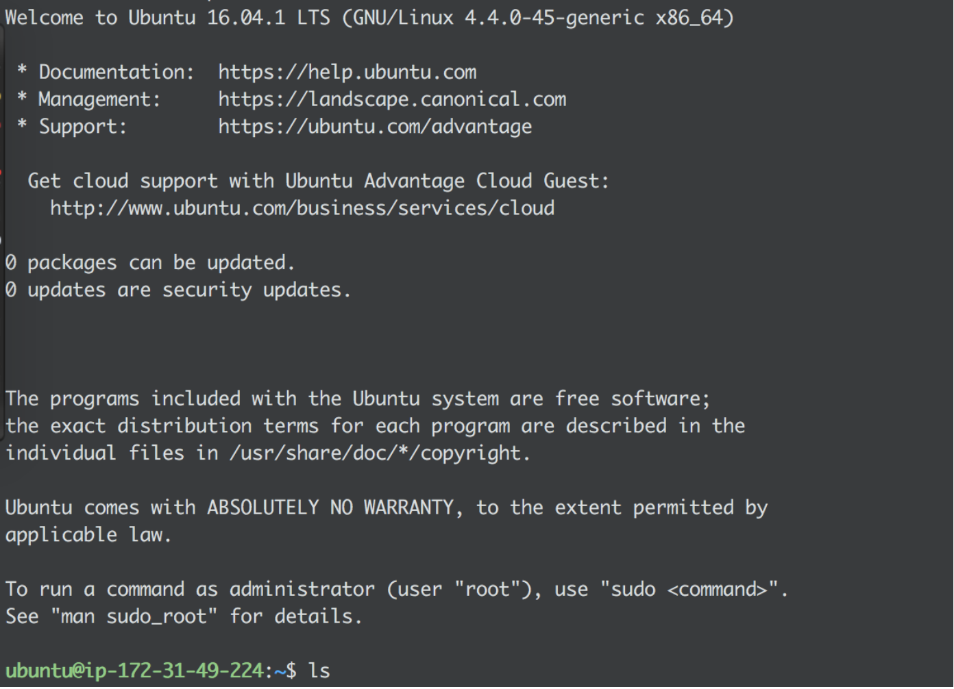
# Upload the dataset to the instance from a local terminal
scp -i ~/.ssh/RandomKey.pem ~/path_to_datafile/RC_2015 -01.bz2 ubuntu@ec2 -54-165-250-39.compute -1.amazonaws.com:~/data/RC_2015 -01. bz2

Install dependencies to the instance in order to wrangle the data from distance using the server’s processing power. Firstly we need to download Anaconda to the instance.
# Download Anaconda to the server from a server terminal
wget https://repo.continuum.io/archive/Anaconda2-4.2.0-Linux-x86_64. sh

# Install Anaconda to the instance from a server terminal
bash Anaconda2-4.2.0-Linux-x86_64.sh

Settle a server ipython notebook for remote handling python reports and querying data.
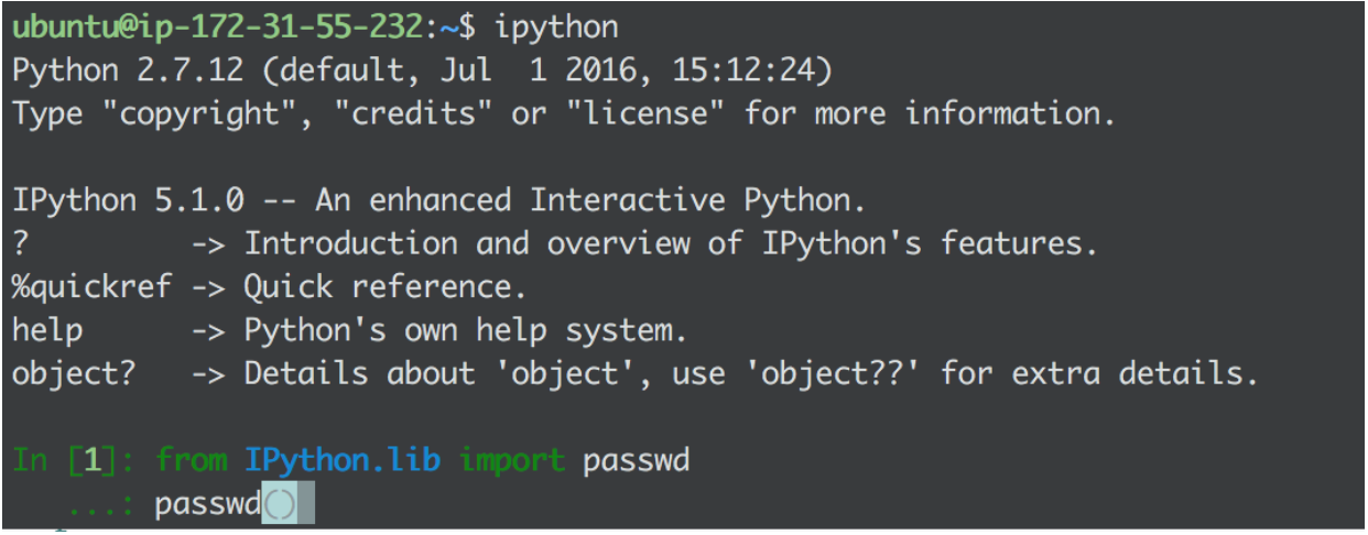
# Open ipython in server environment and do the following command
ipython

# It will prompt a python interactive window that works in the bash environment
# Then create a password by typing the below commands
from IPython.lib import passwd passwd ()

# You will be prompted to enter and verify a password
# (You should remember it. This will be the password to log to the remote ipython notebook)
# When done copy the generated sha1 key
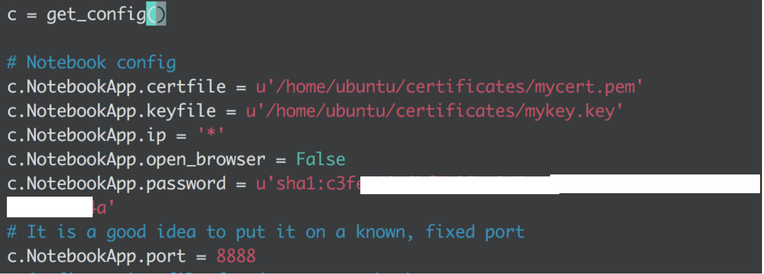
Locate the ipython_notebook_config.py file in the .jupyter directory of the server and paste the key in the appropriate field along with the rest of the uncommented lines.
# If you don’t already have a ipython_notebook_config.py file create one using the below command
jupyter notebook --generate -config
Now the connection is established.
# Write the below command to launch ipython
ipython notebook
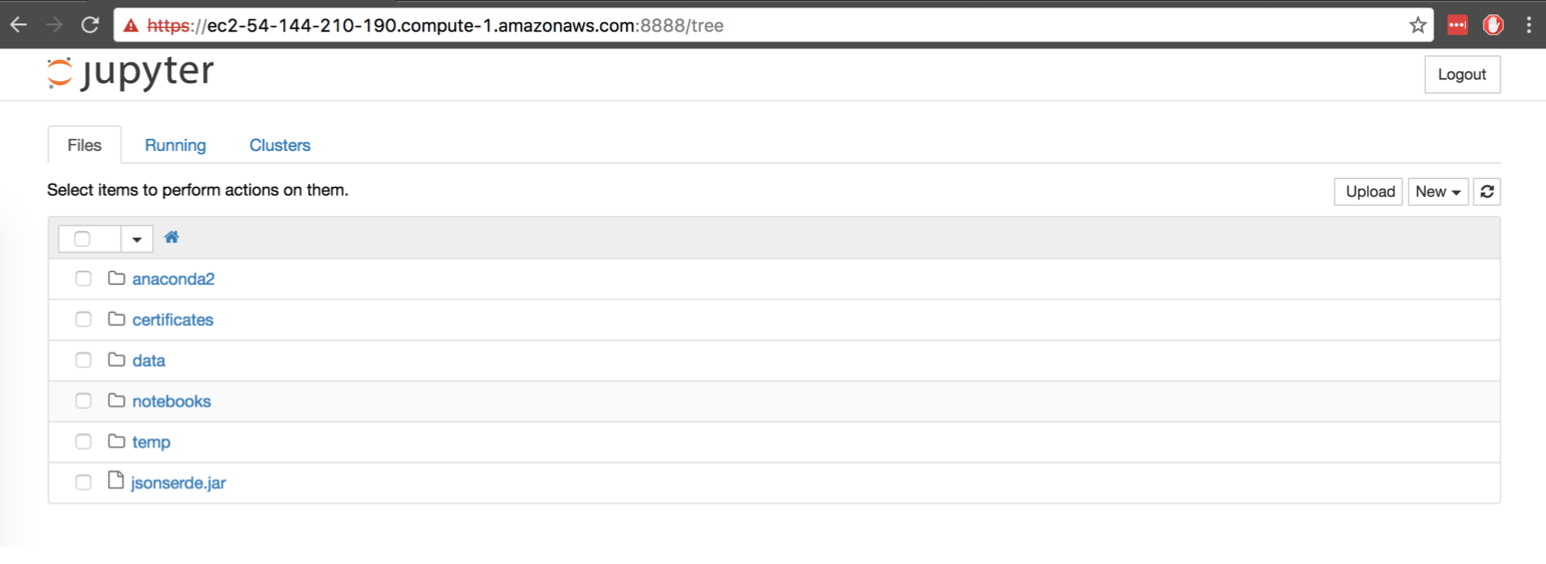
You will be prompted to open a browser. You should write
https://[ip adress of the server]:[port]
Step 2 - Extract data and start data wrangling
Now that we have set everything up, we are ready to parse the data with ipython notebook remotely. We will use Dask and Castra. From now on we write code directly to server’s notebook as mentioned in step 1. Firstly we will load all libraries used on the project. Then we will examine a single row of the dataset with the help of bz2 to parse the compressed file and ujson to load the row.
# Load all libraries used
from bz2 import BZ2File
import ujson
import json
import re
import pandas as pd
from pandas import Timestamp, NaT, DataFrame
from toolz import dissoc
from castra import Castra
from toolz import peek, partition_all
import time
import datetime
import dask.dataframe as dd
import dask.array as da
from dask.diagnostics import ProgressBar
from dask.diagnostics import visualize
from dask.diagnostics import ResourceProfiler
import numpy as np
import nltk
from nltk.corpus import stopwords
import dask.bag as db
from bokeh.charts import TimeSeries, output_notebook, show
from string import punctuation
from itertools import izip
import matplotlib.pyplot as plt
import math
from wordcloud import WordCloud, STOPWORDS
from scipy.misc import imread
with BZ2File(’data/RC_2015-01.bz2’) as f:
    line = f.readline()
ujson.loads(line)
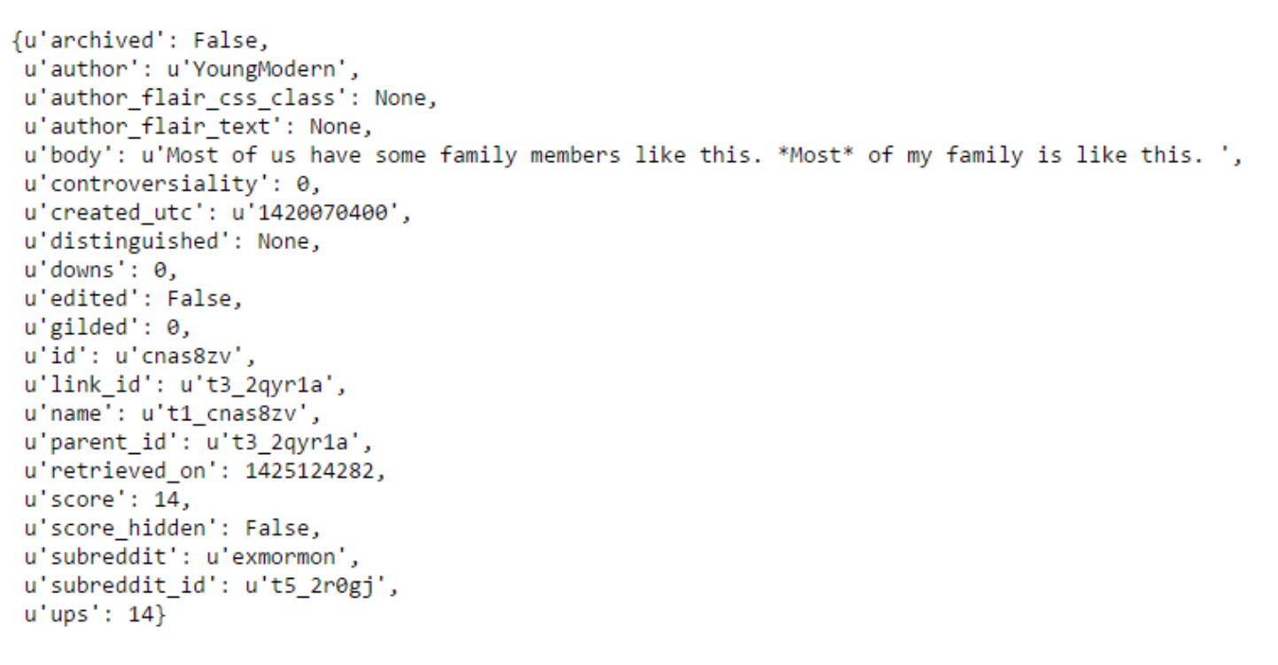
The below block of code is inspred and most of it used by this tutorial for Castra
Now we should create the castra file to parse data on the disk and not on the memory as the memory is not enough to handle such volumes of data.
# Create a path for locating the data files
path = "data"
raw_file = "RC_2015-01.bz2"

# Give a number of lines processed per attempt
# Use a small number because of the small memory size(1GB) of the instance
lppa = 20000
Create functions that will handle the transformation of the json bz2 file into castra files.
#Convert a line of JSON(post) into a cleaned up dict.
def to_json(line):
    post = ujson.loads(line)

    # Convert timestamps into Timestamp objects.
    # It will help us create the sentiment analysis over time date = post["created_utc"]
    post["created_utc"] = Timestamp.utcfromtimestamp(int(date)) edited = post["edited"]
    post["edited"] = Timestamp.utcfromtimestamp(int(edited)) if edited else NaT

    # Convert deleted posts into None values
    if post["author"] == "[deleted]":
        post["author"] = None
    if post["body"] == "[deleted]":
        post["body"] = None

    # Remove "id", and "subreddit_id" as they’re redundant
    # Remove "retrieved_on" as it’s irrelevant
    return dissoc(post, "id", "subreddit_id", "retrieved_on")

# Store the column names for each post in a variable
columns = ["archived", "author", "author_flair_css_class", "author_flair_text", "body", "controversiality", "created_utc", "distinguished", "downs", "edited", "gilded", "link_id", "name", " parent_id", "removal_reason", "score", "score_hidden", "subreddit" , "ups"]

# Convert a list of json strings into a dataframe
def to_df(batch):
    posts = map(to_json, batch)
    df = DataFrame.from_records(posts, columns=columns)
    return df.set_index("created_utc")
Run the code below only if you are sure that you want the castra file with the above requirements to be created. It will cover almost 30GB of space into the disk and will take up to 1,5 hours.
#Creating the castra file
print "Processing.."
start = time.time()
categories = ["distinguished", "subreddit", "removal_reason"]
with BZ2File(path+raw_file) as f:
    batches = partition_all(lppa, f)
    df, frames = peek(map(to_df, batches))
    castra = Castra("reddit_data.castra", template=df, categories=categories)
    castra.extend_sequence(frames, freq="3h")

end = time.time()
print "Castra file has been created in %s:" % str(datetime.timedelta(seconds=(end-start)))

If you don’t have the memory capacity to handle the process, you can use a smaller number of ’lines processed per attempt’ (e.g lppa=5000) and uncomment and run the couple of below blocks of code.
# Create the castra dataset. This will help with I/O operations
'''
def to_castra(fullpath,lppa):
    categories = [’distinguished’, ’subreddit’, ’removal_reason’]
    filename = fullpath.split(’/’)[-1].split(’.’)[0]
    with BZ2File(fullpath) as f:
        batches = partition_all(lppa, f)
        castra = None
        for batch in batches:
            df = to_df(batch)
            if castra == None:
                castra = Castra(path+’reddit_’+filename+’.castra’, template=df, categories=categories)
            castra.extend(df)
'''
'''
print "Processing.."

#Creating the castra file
start = time.time()
to_castra(path+raw_file,lppa)
end = time.time()
print "Castra file has been created in %s:" % str(datetime.timedelta(seconds=(end-start)))
'''
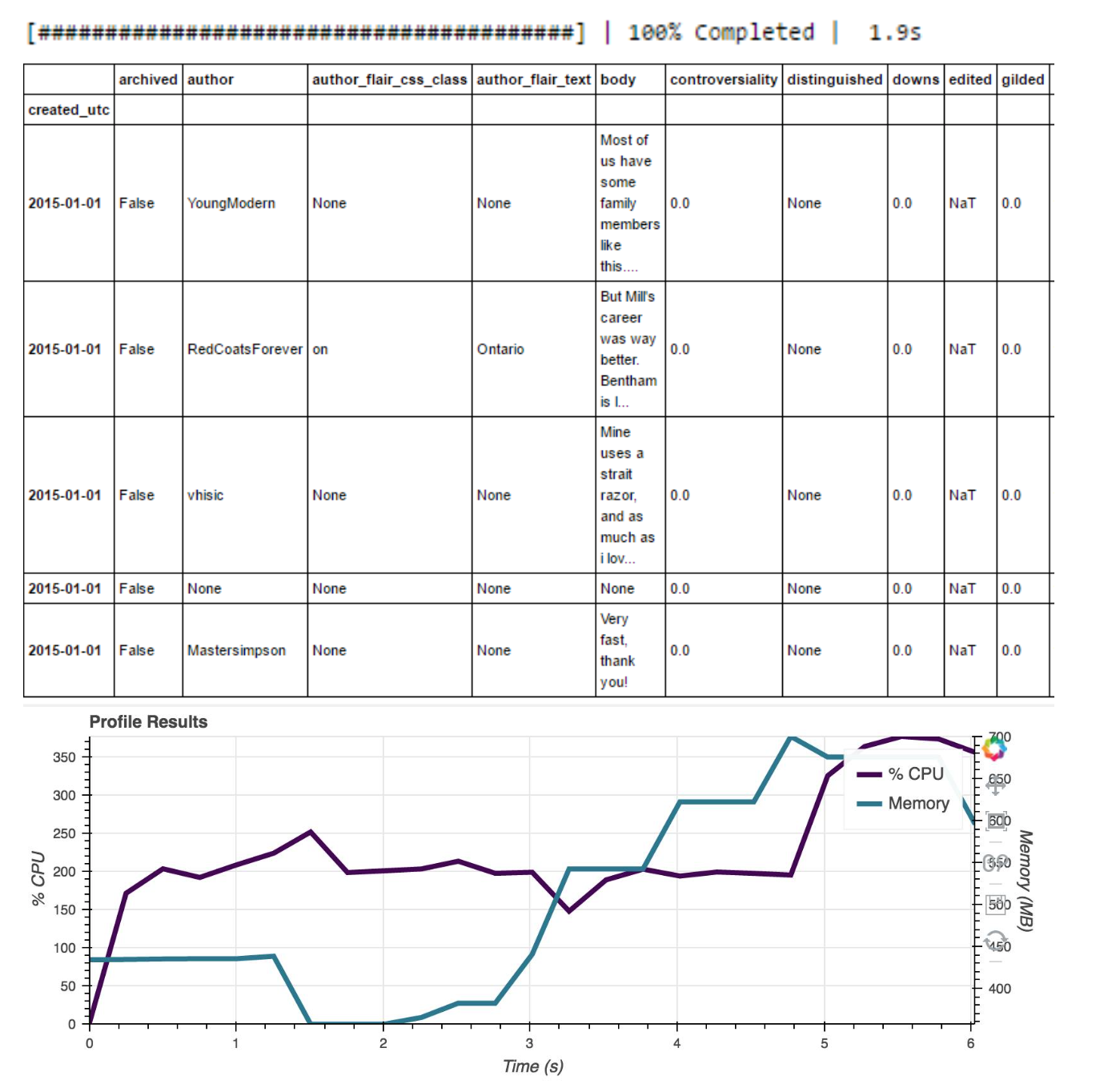
With the castra files created, we can load them into a dask dataframe with the below commands.
# Start ram and CPU visualizer for all computations
a = da.random.random(size=(10000, 1000), chunks=(1000, 1000))
q, r = da.linalg.qr(a)
a2 = q.dot(r)

with ResourceProfiler(dt=0.25) as rprof:
    out = a2.compute()
rprof.visualize()

# Start a progress bar for all computations
pbar = ProgressBar()
pbar.register()

# Load data into a dask dataframe:
path_castra = "data/reddit_RC_2015-01.castra"
df = dd.from_castra(path_castra, columns=columns)
df.head(5)
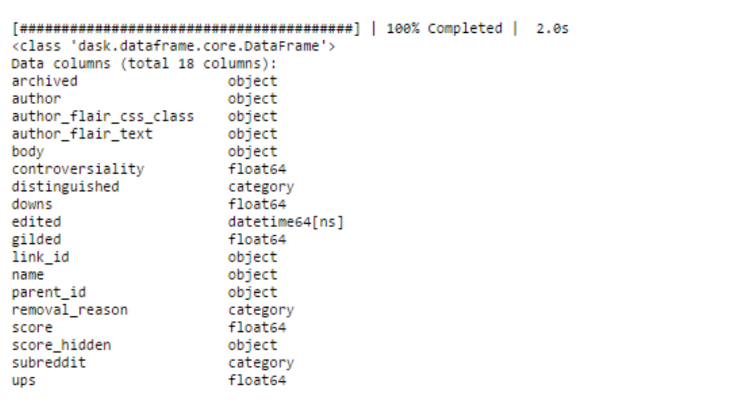
Let’s do some basic computations to have a look on the dataset
# General info about the dataset
df.info()
# The total number of posts
df.downs.count().compute()

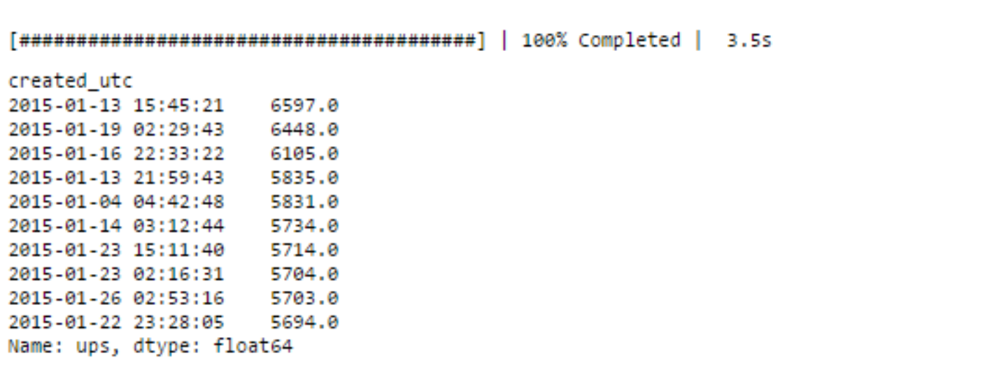
# Top 10 up-rated values
df.ups.nlargest(10).compute()
# Cell counts for the top 10 subreddits
df.groupby("subreddit").count().nlargest(10).compute()
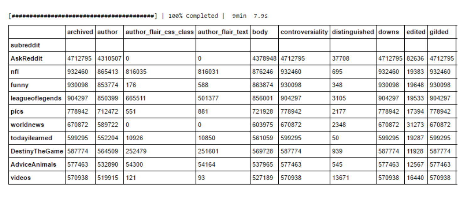
# The posts with ups>5000
df[df[’ups’]>5000].compute()
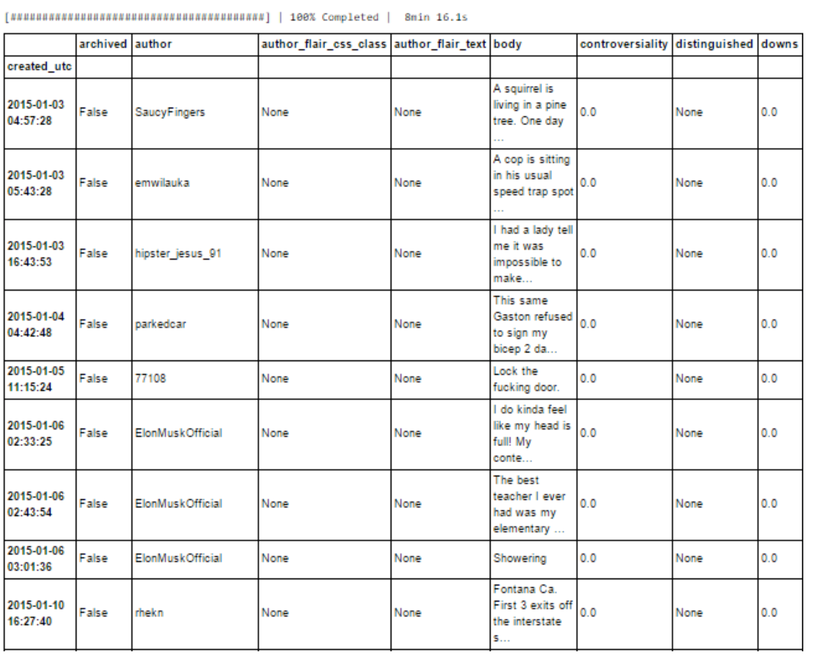
# Create a Series with number of counts per 12 hours
counts_12h = df.ups.resample(’12h’).count().compute()

# Create a lineplot
plt.figure(num=1,figsize=(12, 8), dpi=80)
line, = plt.plot(counts_12h.index, counts_12h.values, lw=2)
plt.axis()
plt.xlabel("Date")
plt.ylabel("Posts") plt.title("All Comments")
plt.show()
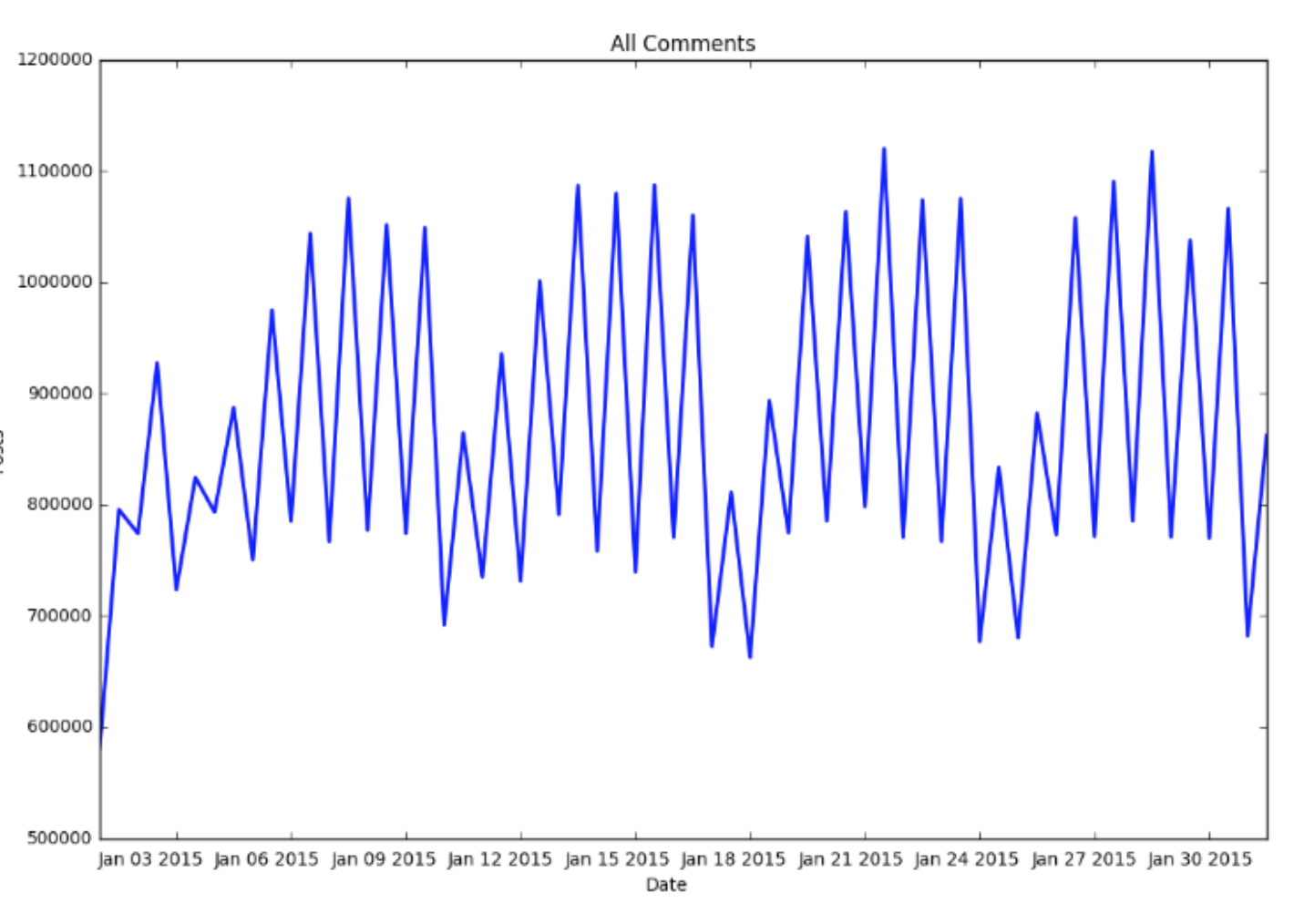
Each point of the above linegraph is the total number of posts within a 12 hour sequence between each point. It shows the difference on post frequency between the western and eastern hemisphere. Reddit is well known at the western hemisphere, that’s why there is a big difference between two consecutive posts. In addition one can see that every 10 points (5 days) there are 4 points with lower frequency. These are the weekends.
Now it is time to take a look at the body of each post.
Step 3 - Sentiment Analysis over time
The below list was generated by users on Mechanical Turk. It is a tab-delimited file named Data Set S1, with a set of 10,222 words, with information about their average happiness evaluations. The words are ordered according to average happiness (descending), and the file contains eight columns: (1) word, (2) rank, (3) average happiness (50 user evaluations), (4) standard deviation of happiness, (5) Twitter rank, (6) Google Books rank, (7) New York Times rank, (8) Music Lyrics rank. The last four columns correspond to the ranking of a word by frequency of occurrence in the top 5000 words for the specified corpus. A double dash ‘–’ indicates a word was not found in the most frequent 5000 words for a corpus.
Let’s firstly take a look at the Data Set S1 file just to have an idea of what this is all about.
# Load first 5 lines of file
columns = ["word", "happiness_rank", "happiness_avg", "happiness_std" , "twitter_rank", "google_rank", "nyt_rank", "lyrics_rank"]
happy_file = pd.read_csv("data/Data_Set_S1.txt", sep="\t", names= columns, encoding="latin-1")[1:]
happy_file.head()

# Change data type to numeric
happy_file[["happiness_avg"]]= happy_file[["happiness_avg"]].apply( pd.to_numeric)
# Happiness average value range
print "happiness value range : { %f - %f } \nmean \t\t\t: { %f }" % \
(happy_file.happiness_avg.min(),happy_file.happiness_avg.max(),
happy_file.happiness_avg.mean())

Secondly we will create a dictionary which will be used as a mapper. Each key will be a word and each value, the average happiness ratio.
# Create happy_dictionary
happy_dict = {}
index = 1
for k in happy_file["word"]:
    happy_dict[k] = happy_file["happiness_avg"][index]
    index +=1
Now that we have the mapper available let’s go back to the reddit posts. We should collect all the bodies, pick the theme(subreddit) we like to analyze, clean its texts(body), tokenize them and create a big bag of words.
# Load castra file into a dask bag
bag = db.from_castra('reddit_data.castra/', columns=['subreddit', 'body'])

# Show a sample of the first post
bag.take(1)

# Save files with subreddit "worldnews"
matches_subreddit = bag.filter(lambda x: x["subreddit"] == "worldnews")

# Collect only the bodies of posts
bodies = matches_subreddit.pluck("body")

# Create a bag of tokens
dirty_bag = bodies.map(nltk.word_tokenize).concat()

# Lower all characters in the bag
lower_bag = dirty_bag.map(lambda x: x.lower())

# Clean bag from stopwords
clean_bag = lower_bag.filter(lambda x: x not in stopwords.words("english"))

# keep only alphanumeric characters as words in the bag and remove NoneType
bag_of_words = clean_bag.filter(lambda x: re.search("^[0-9a-zA-Z]+$", x) is not None)
print "Processing.."
start = time.time()

# Keep all of the above in a variable in memory by using .compute()
bag_of_words = bag_of_words.compute()

end = time.time()
print "The bag of words has been created in: %s" % str(datetime.timedelta(seconds=(end-start)))

# Save bag_of_words to a file to release cache memory usage
with open("data/bag_of_words.csv", "w") as f:
    for item in bag_of_words:
        f.write("%s\n" % item)
# Restart kernel and load the file again
with open("data/bag_of_words.csv", "r") as f:
    bag_of_words = [item[:-1] for item in f]
# Print no. of words in the bag
print 'No. of words in the bag: ', len(bag_of_words)

Now that we have a bag of words, we can create the functions that will iterate in each word, check the happiness_avg if there is any, create a sliding windows of 500 words and check the sentiment analysis results.
def happy_meter(tokens):
    # Check if tokens match happy_dict counter = 0
    total_ratio = 0
    for i in happy_dict.keys():
        for token in tokens:
            if token in i:
                counter+=1
                total_ratio+=float(happy_dict[i])

    # print "Happiness ratio range is (1.30 - 8.50)"
    if counter == 0:
        return 0 #"There are no words with sentiment attached"
    else:
        return total_ratio/counter
        #"The happiness ratio of this text is: {0:.2f}".format(total_ratio/counter)
def sentimentizer(bag,n):

    # Create buckets of words
    buckets = izip(*[iter(bag)]*n)

    # Calculate sentiment of each bucket and assign values to new dictionary
    counter = 1
    ratio = []
    word_counter = []
    for bucket in buckets:
        ratio.append(happy_meter(list(bucket)))
        word_counter.append(n*counter)
        counter+=1

    # Create a lineplot for sentiment profile
    plt.figure(num=1,figsize=(12, 8), dpi=80)
    line, = plt.plot(count_12h.index, ratio, lw=2)
    plt.axis()
    plt.xlabel(’Date’)
    plt.ylabel(’Happiness Ratio’) plt.title(’Sentiment Profile’)
    plt.show()
# Create profiles for sliding windows of length 500 words
# It takes almost 4 hours to run!!
sentimentizer(bag_of_words,500)
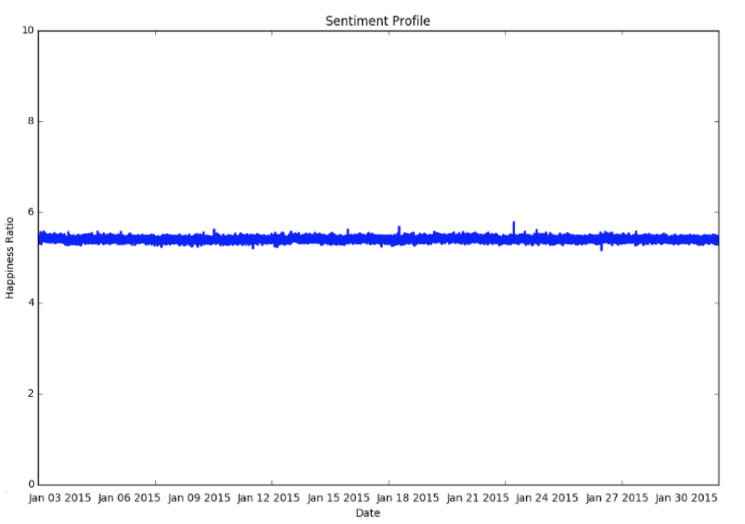
On average, one can tell that January 2015 was generally a neutral month in terms of happiness as it is close to 5.5 which is the mean of average happiness. But we can see some happier peaks (close to 6) on January 23rd. If we had used a sliding window of 50 words, we would have a higher range of values but in order to see the differences in time we should zoom-in the plot. If we have took a bigger sliding window (12 hours) we would have seen a straight line close to 5.5.
Step 4 - WordCloud
Now we will create a word cloud based on the bag of words with subreddit ‘worldnews’
# Create a function that turns the bag_of_words into a string
def generate_string(bag):
    s = ''
    s+=' '.join([word for word in bag])
    return s

# Generate string from bag_of_words
s = generate_string(bag_of_words)

# Exclude some more from the cloud
stopwords = {"deleted", "gt"}
STOPWORDS = STOPWORDS.union(stopwords)

# Create a mask as a stencil for the word cloud
world_mask = imread("photos/world_3.jpg",flatten=True)

# Set requirements for the bag_of_words
wc = WordCloud(background_color="white", max_words=2000, width=1800, height=1400, mask=world_mask, stopwords=STOPWORDS)

# Generate the word cloud by sourcing the string
wc.generate(s)

#  Save the word cloud
#plt.imshow(wc)
plt.axis("off")
plt.savefig("photos/world_cloud.png", dpi=300)
plt.figure(figsize=(12,8),dpi=500)
img=plt.imshow(wc)
#plt.imshow(world_mask, cmap=plt.cm.gray)
plt.axis("off")
plt.show()
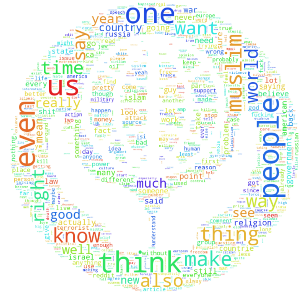
One can see that the top words of the cloud are: people, one, think, even and Muslim. The latter is due to the terrorist attacks occurred from 7 January 2015 to 9 January 2015, across the Île-de-France region, particularly in Paris. Three attackers killed a total of 17 in four shooting attacks, and police then killed the three assailants.